Assembling data

• What constitutes a good assembly?

• How to estimate assembly quality

• Co-assembly

These instructions assume you are using the EBI Training Virual Machines. If you’re running this on your own computer instead, remember that some file paths will be different. In particular, /home/training/ will be /home/<yourusername>.

Assembly and Co-assembly

 Learning Objectives - in the following exercises you will learn how to perform a metagenomic assembly and to start some basic analysis of the output. Subsequently, we will demonstrate the application of co-assembly. Note, due to the complexity of metagenomics assembly, we will only be investigating very simple example datasets as these often take days of CPU time and 100s of GB of memory. Thus, do not think that there is an issue with the assemblies.

Once you have quality filtered your sequencing reads, you may want to perform de novo assembly in addition to, or as an alternative to a read-based analyses. The first step is to assemble your sequences into contigs. There are many tools available for this, such as MetaVelvet, metaSPAdes, IDBA-UD, MEGAHIT. We generally use metaSPAdes, as in most cases it yields the best contig size statistics (i.e. more continguous assembly) and has been shown to be able to capture high degrees of community diversity (Vollmers, et al. PLOS One 2017). However, you should consider the pros and cons of different assemblers, which not only includes the accuracy of the assembly, but also their computational overhead. Compare these factors to what you have available. For example, very diverse samples with a lot of sequence data uses a lot of memory with SPAdes. In the following practicals we will demonstrate the use of metaSPAdes on a small sample and the use of MEGAHIT for performing co-assembly.

 Let’s first change to the working directory where we will be running the analyses:

cd /home/training/Data/Assembly/files

 To run metaspades you would execute the following commands (but don’t run it now!):

mkdir assembly
metaspades.py -t 4 --only-assembler -m 10 -1 reads/oral_human_example_1_splitaa_kneaddata_paired_1.fastq -2 reads/oral_human_example_1_splitaa_kneaddata_paired_2.fastq -o assembly

 Since the assembly process would take ~1h we are just going to analyse the output present in assembly.bak. Let’s look at the contigs.fasta file.

For this, take the first 40 lines of the sequence and perform a blast search at NCBI (https://blast.ncbi.nlm.nih.gov/Blast.cgi, choose Nucleotide:Nucleotide from the set of options). Leave all other options as default on the search page. To select the first 40 lines of the assembly perform the following:

head -41 assembly.bak/contigs.fasta

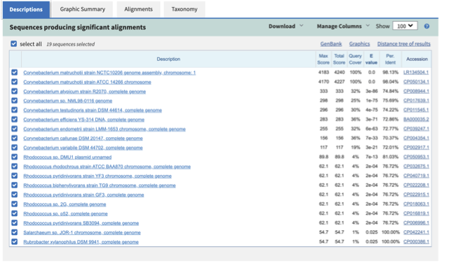
 Which species do you think this sequence may be coming from? Does this make sense as a human oral bacteria? Are you surprised by this result at all?

Now let us consider some statistics about the entire assembly

assembly_stats assembly.bak/scaffolds.fasta

 This will output two simple tables in JSON format, but it is fairly simple to read. There is a section that corresponds to the scaffolds in the assembly and a section that corresponds to the contigs.

 What is the length of longest and shortest contigs?

 What is the N50 of the assembly? Given that are input sequences were ~150bp long paired-end sequences, what does this tell you about the assembly?

 N50 is a measure to describe the quality of assembled genomes that are fragmented in contigs of different length.  We can apply this with some caution to metagenomes, where we can use it to crudely assess the contig length that covers 50% of the total assembly.  Essentially the longer the better, but this only makes sense when thinking about alike metagenomes. Note, N10 is the minimum contig length to cover 10 percent of the metagenome. N90 is the minimum contig length to cover 90 percent of the metagenome.

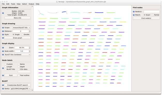
 Bandage (a Bioinformatics Application for Navigating De novo Assembly Graphs Easily), is a program that creates interactive visualisations of assembly graphs. They can be useful for finding sections of the graph, such as rRNA, or to try to find parts of a genome. Note, you can install Bandage on your local system. With Bandage, you can zoom and pan around the graph and search for sequences, plus much more. The following guide allows you to look at the assembly graph.  Normally, I would recommend looking at the ‘ assembly_graph.fastg, but our assembly is quite fragmented, so we will load up the assembly_graph_after_simplification.gfa.

At the terminal, type

Bandage

In the the Bandage GUI perform the following

Select File -> Load graph

Navigate to Home -> Data -> Assembly -> files -> assembly.bak and open the file assembly_graph_after_simplification.gfa

Once loaded, you need to draw the graph. To do so, under the “Graph drawing” panel on the left side perform the following:

Set Scope to ‘Entire graph’

The click on Draw graph

 Use the sliders in the main panel to move around and look at each distinct part of the assembly graph.

 Can you find any large, complex parts of the graph? If so, what do they look like.

In this particular sample, we believe that strains related to the species Rothia dentocariosa, a Gram-positive, round- to rod-shaped bacteria that is part of the normal community of microbes residing in the mouth and respiratory tract, should be present in our sample. While this is a tiny dataset, lets try to see if there is evidence for this genome. To do so, we will search the R. dentocariosa genome against the assembly graph.

To do so, go to the ‘BLAST’ panel on the left side of the GUI.

Step 1 - Select ‘Create/view BLAST search’, this will open a new window

Step 2 - Select ‘build Blast database’

Step 3 - Load from FASTA file. Navigate to the genome folder: Home -> Data -> Assembly -> files -> genome and select GCA_000164695.fasta

Step 4 - Modify the BLAST filters to 95% identity

Step 5 - Run BLAST

Step 6 - Close this window

To visualise just these hits, go back to “Graph drawing” panel.

Set Scope to ‘Around BLAST hits’

Set Distance 2

The click on ‘Draw graph’

You should then see something like this:

 In the following steps of this exercise, we will look at performing co-assembly of multiple datasets. Each should take about 15-20 min. In case you do not manage to finish these on time, the directory coassembly.bak contains all the expected results.

 First, we need to make sure the output directories we are going to create do not already exist (MEGAHIT cannot overwrite existing directories). Run:

rm -rf coassembly/assembly*

 Then, perform the coassemblies with MEGAHIT, as follows:

megahit -1 reads/oral_human_example_1_splitac_kneaddata_paired_1.fastq -2 reads/oral_human_example_1_splitac_kneaddata_paired_2.fastq -o  coassembly/assembly1 -t 4 --k-list 23,51,77

megahit -1 reads/oral_human_example_1_splitac_kneaddata_paired_1.fastq,reads/oral_human_example_1_splitab_kneaddata_paired_1.fastq  -2 reads/oral_human_example_1_splitac_kneaddata_paired_2.fastq,reads/oral_human_example_1_splitab_kneaddata_paired_2.fastq -o coassembly/assembly2 -t 4 --k-list 23,51,77

megahit -1 reads/oral_human_example_1_splitab_kneaddata_paired_1.fastq,reads/oral_human_example_1_splitac_kneaddata_paired_1.fastq,reads/oral_human_example_1_splitaa_kneaddata_paired_1.fastq -2 reads/oral_human_example_1_splitab_kneaddata_paired_2.fastq,reads/oral_human_example_1_splitac_kneaddata_paired_2.fastq,reads/oral_human_example_1_splitaa_kneaddata_paired_2.fastq -o coassembly/assembly3 -t 4 --k-list 23,51,77

 You should now have three different assemblies, let us compare the results.

assembly_stats coassembly/assembly1/final.contigs.fa
assembly_stats coassembly/assembly2/final.contigs.fa
assembly_stats coassembly/assembly3/final.contigs.fa

How do these assemblies differ to the one generated previously with metaSPAdes? Which one do you think is best?